drifft¤

drifft computes allele-count distributions under the discrete-time Wright–Fisher model, with selection, mutation, and changing population sizes. It evaluates probability distributions deterministically rather than simulating individual trajectories. You can compute loss and fixation probabilities, expectations, and expected visits before absorption, and differentiate results with respect to selection, mutation, or initial mass using JAX.

The numerical algorithms target the discrete-time binomial transition. Their approximations accelerate that calculation without replacing it by a diffusion model. Population sizes and generation counts are fixed inputs, not differentiable parameters.

Compose the model, choose the computation¤

drifft separates the biological model from its numerical implementation. Frequency maps map parental allele frequency to offspring sampling probability after selection and mutation, and can be composed in the order the processes occur. Demographic histories describe how population size changes over time.

Backends are numerical representations of one-generation transitions; evolution methods apply them across longer intervals. A backend precomputes grids and weights for fixed population sizes and numerical settings, so these quantities can be reused as biological parameters change. The computational overview explains the tasks and approximation structure before introducing individual algorithms.

Installation¤

drifft requires Python 3.12 or newer. From a repository checkout:

git clone https://github.com/mancusolab/drifft.git
cd drifft
uv sync

Run Python scripts with uv run python. All backends require float64; enable jax_enable_x64 before constructing a backend, as shown below.

Quickstart¤

What is the probability that a new deleterious allele is lost in the next generation, and how does that probability change with selection?

Run this example with uv run python:

import jax
import jax.numpy as jnp
import drifft

jax.config.update("jax_enable_x64", True)

# 32 diploid individuals carry 64 gene copies.
backend = drifft.FFT(gene_copies=64)
selection = drifft.AdditiveSelection(s_het=0.01)
transition = drifft.Transition(backend, frequency_map=selection)

# Exactly one copy of the derived allele is present initially.
initial = jnp.zeros(65).at[1].set(1.0)
after_one_generation = transition.advance(initial)
print(f"Loss probability: {after_one_generation[0]:.4f}")

The three genotype fitnesses are \((1,0.99,0.98)\). The returned array describes all possible offspring counts: entry zero is loss, entry 64 is fixation, and entries 1 through 63 represent a segregating allele. The loss probability is about 0.37: an allele starting from a single copy has a substantial chance of disappearing through random reproduction in the next generation.

Differentiate the result¤

Put the same calculation in a function of the selection coefficient and apply jax.grad:

def loss_probability(s_het):
    selected = drifft.Transition(
        backend, drifft.AdditiveSelection(s_het=s_het)
    )
    return selected.advance(initial)[0]

sensitivity = jax.grad(loss_probability)(jnp.asarray(0.01))
print(f"Sensitivity to s_het: {sensitivity:.4f}")

The derivative is positive: increasing the fitness penalty makes immediate loss more likely. The calculation reuses the prepared backend while selection changes.

Multiple generations¤

Reuse the selection model, compose it with mutation, and supply a population history and evolution method:

frequency_map = drifft.Composition(
    selection,
    drifft.Mutation(forward_rate=1e-5, backward_rate=1e-5),
)
history = drifft.Demography(ne=[32, 16, 32], generations=[20, 20])
model = drifft.DemographicTransition(
    history,
    frequency_map=frequency_map,
    backend=drifft.FFT,
    method=drifft.Sequential(),
)
result = model.advance(initial)
print(f"Probability of zero copies after 40 generations: {result.distribution[0]:.4f}")

Composition applies selection first, then mutation. Each demographic interval holds its source size until its final generation, when the population changes size. Here, backend is a factory: drifft prepares geometry for each distinct population size. The frequency map and method are reused across the history.

The same history and frequency map can be used with other numerical components. See choosing numerical algorithms for the available combinations and accuracy and differentiation for validation.

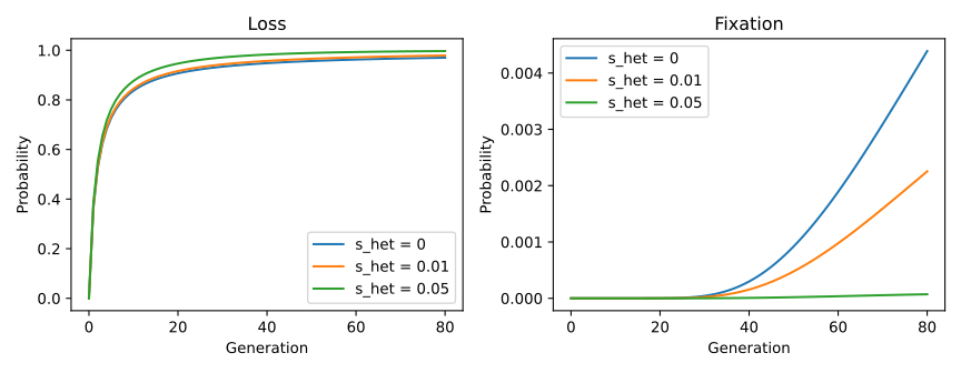
The allele-loss example extends the calculation to 80 generations and compares three selection strengths. The bottleneck example uses changing population sizes.

Computation¤

Wright–Fisher transition distributions are concentrated around their means, and nearby offspring probabilities produce similar distributions. drifft uses this structure in its optimized backends to compute transitions without storing the full matrix. Dense provides an independent reference for small populations. The name combines genetic drift and the FFT. Fast transforms accelerate one-generation transitions. Polynomial compression and Krylov methods can reduce the work across long constant-size intervals.

Dependencies and hardware¤

jax-finufft is a core dependency for NUFFT. The project uses its Git version, with the exact commit recorded in uv.lock. Installing from Git builds the native extension and requires a C++ toolchain. The build uses installed FFTW development libraries when available; otherwise it downloads and builds FFTW automatically (OpenMP is optional). Ubuntu CI installs libfftw3-dev to avoid that extra build. CPU execution is tested on Apple Silicon. CUDA requires a compatible CUDA-enabled FINUFFT installation and has not been validated here; TPU is unsupported. No dense fallback is used when a device lacks NUFFT support.